In this article, I will provide a complete walk through of a popular concept in data science interviews - the confidence interval, from its intuition, definition to actual computation.
Intuition
When encountering a new concept, my natural impulse would be to ask the question: how does this concept help in solving real world problem? This concept is introduced to answer the question below: > How to use sample mean to deduce population mean and quantify our certainty? > > Or rather, how can we use sample means with some degree of certainty?
What is a confidence interval?
Let's set up a fake scenario to see how this means in practical context. Suppose you want to investigate the population's average height \(\mu\) on a island (10,000 people in total). You already obtained a sample with 100 people's height recorded, how to give a quantify the certainty of a population mean deduction? That is to say, we want to obtain a bound for the population mean: \[ \text{lower limit} < \mu < \text{upper limit} \]
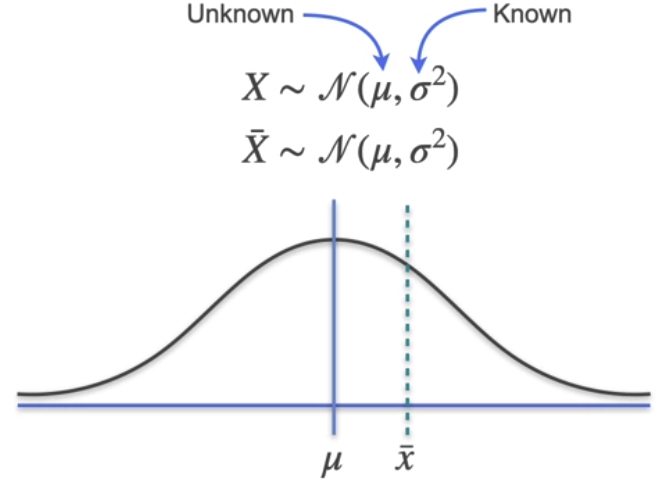
This interval is the confidence interval I want to introduce in this article. To make things simple, let's assume that heights on this island follow a normal distribution with a mean \(\mu\), which is unknown, and a population variance, \(\sigma^2\), which for now will assume is known (\(X \sim \mathcal{N}(\mu, \sigma^2)\)). This may seem weird to know \(\sigma\) without knowing \(\mu\), but it simplifies the problems for now and we will see how to deal with unknown variance later.
To generate such a confidence interval, a random sample needs to be taken from the population. To further simplify the setting, we start with a sample of size one. Since the sample has only one person in it, their height will also be the sample mean, which will be called \(\bar x\). Let's create a random variable, \(\bar X\), to describe the probability of selecting different sample means. It's actually going to be identical to the population (\(X\)), a normal distribution centered of \(\mu\) with a variance \(\sigma^2\). (\(\bar X \sim \mathcal{N}(\mu, \sigma^2)\)). This doesn't mean you suddenly know the true value of \(\mu\), but you do know \(X\) and \(\bar X\) have the same mean.

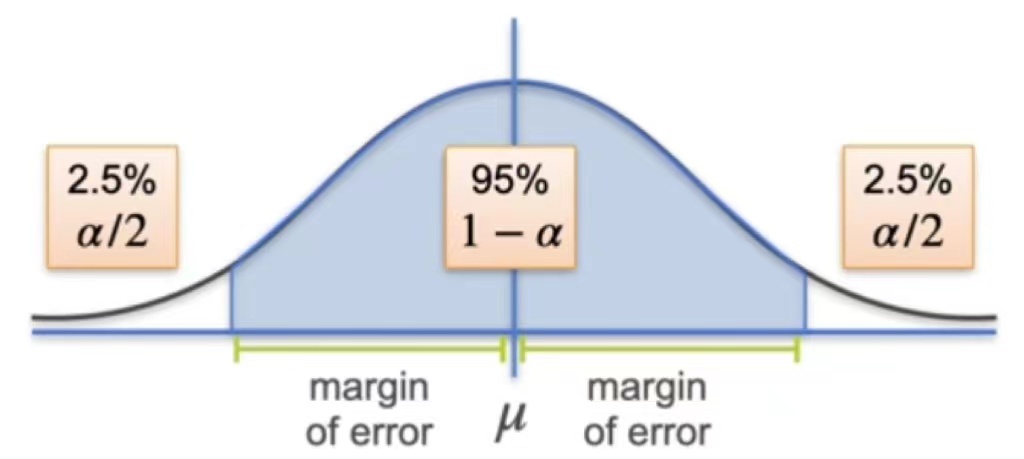
With this setting, as we can't know for sure whether \(\bar X\) is smaller or larger than the \(\mu\), we do know "How far are most sample means from \(\mu\)?" based on the distribution property. To do this, you need two related concepts. The first one is margin of error, which is a distance on either side of mu, and a confidence level, which is the probability that your sample mean is within that margin of error. To set these two values, you actually normally start with a third one called the significance level, which is denoted with a Greek letter \(\alpha\). In practice, \(\alpha\) is usually set to be \(0.05\), and the confidence level \(1-\alpha\) yield 0.95, also denoted as \(95\%\). This is the probability that a randomly generated sample mean falls within the margin of error. Since the normal distribution is symmetric around its mean, you can say that 2.5% (\(\alpha\)) of the time your sample mean will lie outside the margin of error because it's too big and 2.5% of the time because it's too small.

What does the confidence level stands for?
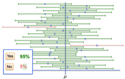
Given \(n=1\), Known \(\sigma\) and defined margin of error \(95\%\), when we sample multiple times, there will be approximately 95% of the chance that our confidence interval contains the population mean \(\mu\). Here is a graph illustration of what confidence level stands for. Where we sample multiple times and the green interval suggest the population mean \(\mu\) is in the interval while red interval suggest it does not. In other words, with a confidence level, we could say that the confidence interval contains the true population parameter approximately 95% of the time.

What is the effect of changing sample size?
We made an simplification to use an sample of size 1 in the previous chapters, you may be wondering how things will change if we change the size of that?
First, we need to know, \(\mu_{\bar{x}}\), or the expected value of the sample mean, always equals \(\mu\), the population mean. This is true no matter how many observations are in your sample. Now consider the standard deviation of the sample mean, \(\sigma_{\bar{x}}\). We know that it will be equal to the population standard deviation divided by the square root of the number of samples, n, which is (\(\sigma / \sqrt{n}\)). In this case, it does vary with sample size.
Then whats the effect of changing sample size? You may find as the \(n\) increase, the fraction \(\frac{\sigma}{\sqrt{n}}\) becomes smaller. For a normal distribution, shrinking the standard deviation means the values are more likely to appear near \(\mu\), the central part of the graph.

More generally, as n, the sample size increases, the confidence interval shrinks. In other words, as we collect more data, you can make more precise estimates of \(\mu\) without dropping your confidence level.
Definitions and Calculation Steps
Margin of error
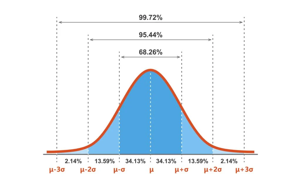
Before dive to the calculation formula, we still need to figure out how to calculate the margin of error. Since we are trying to land 95% of our guesses, we are actually seeking an interval that includes the 95% of the area on the distribution graph. Given a distribution like \(X\sim \mathcal{N}(\mu, \sigma^2)\):

We could conclude from the above image that to include 95% of the area, we are actually trying to get the interval \((\mu-2\sigma, \mu+2\sigma)\). If you know the standard deviation of a normal distribution, you can establish the range around \(\mu\) in which any percentage of the distribution lies. These points that are a specified number of standard deviation away from the mean (the parameter before \(\sigma\) in the upper graph) have a special name, z-scores or z-statistics.
The name z-score is taken from the standard normal distribution, which is often called the z-distribution. You can easily convert normal distributions to the standard normal by subtracting the mean and dividing by the standard deviation. Notice that, when using the z-distribution, the z-scores are simply the value of the point. \[\frac{X-\mu}{\sigma} = Z \sim \mathcal{N} (0,1)\] If you want exactly 95% of the distribution, then the z-scores to two decimal places are \(-1.96\) and \(+1.96\). These two values are called critical values, denoted as \(z_{0.025}\) and \(z_{0.975}\). They are cut-off points inside of which an exact percentage of a probability distribution is contained. To find these values, you'd either look them up in a pre-computed lookup table or use a software library.
Returning back to the non-standardized normal distribution, we can still use these critical values, but since the distribution isn't normalized, we need to multiply them by the standard deviation. Note we also need to take the effect of sample size into account, so the calculation for margin of error should be:
\[ \text{margin of error} = z_{1-\alpha/2} \cdot \frac{\sigma}{\sqrt{n}} \] ### With Unknown Standard Deviation
You may have noticed that the above calculation are based on known standard deviation \(\sigma\), what happens when we don't have access to this measurement? Let's quickly review the process we went through when the standard deviation is known: We are calculating the margin of error by multiplying z-scores with standard deviation, where \(\large \frac{\bar{x}-\mu}{\frac{\sigma}{\sqrt{n}}}\) follows a normal distribution. Now with a unknown \(\sigma\), we can use the sample's deviation \(s\) to replace \(\sigma\), however, random variable \(\large \frac{\bar{x}-\mu}{\frac{s}{\sqrt{n}}}\) no longer follows a normal distribution, it's now a student's t distribution. Instead of continue using the z-value as critical value, we now use t-value which is sampled from the student's t distribution.
\[ \text{margin of error} = t_{1-\alpha/2} \cdot \frac{s}{\sqrt{n}} \]
Confidence intervals for proportion
The above intervals are all calculated for population mean, what about for proportions?
Similarly, we are applying the confidence interval as:
\[\begin{align} \text{Confidence Interval} &= \text{Sample Proportion}\ \pm \ \text{Margin of Error}\\ &=\hat{p}\ \pm\ z_{1-\alpha/2} \cdot \sqrt{\frac{\hat {p} (1-\hat{p})}{n}} \end{align} \]
Summary
In summary, the confidence intervals are calculated using the formula and steps below: \[ \begin{align} \text{Confidence Interval} &= \text{Sample Mean}\ \pm \ \text{Margin of Error}\\ &= \bar{x}\ \pm z_{1-\alpha/2}\cdot {\frac{\sigma}{\sqrt{n}}}\quad \text{(known std)}\\ &=\bar{x}\ \pm t_{1-\alpha/2} \cdot \frac{s}{\sqrt{n}}\quad \text{(unknown std)}\\ &=\hat{p}\ \pm\ z_{1-\alpha/2} \cdot \sqrt{\frac{\hat {p} (1-\hat{p})}{n}} \end{align} \]
- Find the sample mean
- Define a desired confidence level (\(1-\alpha\))
- Get the critical value (\(z_{1-\alpha/2}\))
- Find the standard error \(\left(\frac{\sigma}{\sqrt{n}}\right)\)
- Find the margin of error by multiplying critical value and standard error
- Add/Subtract the margin of error to the sample mean (applying the above formula)
Applications
Now let's look at some concrete examples on how to apply the concepts in practice.
Calculating confidence intervals
Suppose you have a 6,000 population that you want to study the population mean of height. You took a random sample among this population with a size of 49 people and get the following statistics: \(\bar{x} = 170cm, \sigma = 25cm\). Suppose you want a confidence level of 95%, where you know the \(z_{1-{\alpha/2}} = 1.96\).
To calculate the confidence interval, you apply the formula:
\[\begin{align} \text{Confidence Interval} &= \text{Sample Mean}\ \pm \ \text{Margin of Error}\\ &= \bar{x}\ \pm z_{1-\alpha/2}\cdot {\frac{\sigma}{\sqrt{n}}}\quad \text{(known std)}\\ &= 170\ \pm 1.96 \cdot \frac{25}{\sqrt{49}}\\ &=170\ \pm \ 7\\ &= (163cm,177cm) \end{align} \] That is to say, population mean will lies in this interval 95% of the time.
Calculating Sample size
Sometimes we may need to shrink the interval we are having. That is equivalent to say we are trying to reduce the margin of errors by collecting more samples.
Let's continue with the set-up in the previous section. Now we want a margin of error of \(3cm\). What is the smallest sample size to obtain the desired margin of error?
\[\begin{align} \text{margin of error} = z_{1-\alpha/2} \cdot \frac{\sigma}{\sqrt{n}}\\ 3 = z_{1-\alpha/2} \cdot \frac{\sigma}{\sqrt{n}}\\ 3 \ge z_{1-\alpha/2} \cdot \frac{\sigma}{\sqrt{n}} \\ 3 \ge 1.96 \times \frac{25}{\sqrt{n}}\\ n \ge (\frac{1.96\times 25}{3})^2 \approx 267 \end{align} \] That is to say, we need to collect a sample of size 267 people to obtain such a margin of error.
Common interview questions
- Meta: How would you explain a confidence interval to a non-technical audience? (《Ace the Data Science Interview》 6.2)
- Google: How would you derive a confidence interval for the proabability of flipping heads from a series of coin tosses? (《Ace the Data Science Interview》 6.11)
Reference
- Most of the images are taken from Coursera course - Probability & Statistics for Machine Learning & Data Science
- 《Ace the Data Science Interview》 by Kevin Huo & Nick Singh