Complete walk through of general hypothesis testing

In this blog, I will provide a complete walk through of another popular concept in data science interviews - hypothesis testing, from its general setup, key concepts related (test statistics, Type I error, etc.) to actual applications.

General setup

The process of testing whether or not a sample of data supports a particular hypothesis is called ==Hypothesis Testing==.

1. State a null hypothesis (baseline) and an alternative hypothesis (the statement you want to prove).
   • Either the null hypothesis will be rejected (in favor of the alternative hypothesis), or it will fail to be rejected (although failing to reject the null hypothesis does not necessarily mean it is true, but rather that there is not sufficient evidence to reject it)
2. Design your test
   • Decide the Test Statistic to work with
   • Decide the Significance level
3. Compute the observed statistic (based on your sample)
4. Reach a conclusion
   • Compare the p-value to a certain significance level \(\alpha\). (to decide whether to reject or fail to reject your null hypothesis)

Types of hypothesis test

Hypothesis tests are either one- or two- tailed tests. Here \(H_0\) is the null hypothesis and \(H_1\) is the alternative hypothesis, and \(\mu\) is the parameter of interest.

• One tailed tests

\[ \begin{align} H_0:\mu=\mu_0\text{ versus } &H_1:\mu<\mu_0\text{(also called left tailed) }\\ &H_1: \mu>\mu_0 \text{(right tailed)} \end{align} \]

• Two tailed tests \(H_0:\mu=\mu_0\text{ versus } H_1: \mu \ne \mu_0\)

Test statistic

Now lets suppose you have already set up your hypothesis and are marching into step 2 of the setup. Then you may be wondering, what is test statistic?

A ==test statistic== is a numerical summary designed for the purpose of determining whether the null hypothesis or the alternative hypothesis should be accepted as correct. More specifically, it assumes that the parameter of interest follows a particular sampling distribution under the null hypothesis.

Based on the test statistic we select and the assumptions we made with our samples, hypothesis testing varies into different categories. For example, we have:

• Z-test, where we use z-score as the test statistic, and assumes this statistic follows a normal distribution under the null hypothesis. where \(\sigma\) is the population variance and \(\mu_0\) is the population mean.
  • \[z=\frac{\bar{x}-\mu_0}{\sigma/\sqrt{n}}\sim N(0,1)\]
• t-test, where we use a student's t-distribution rather than a normal distribution to cope with unknown population variance.
  • \[t=\frac{\bar{x}-\mu_0}{s/\sqrt{n}}\sim t_{n-1}\]
• Chi-squared test, where we check whether two categorical variables are independent by this test statistic:
  • \[\chi^2=\sum_i\frac{(O_i-E_i)^2}{E_i}\]

There are a lot of other tests not covered like ANOVA, Independent t-test Paired t-test. These tests typically focus on verifying hypothesis with different setup of the samples and population.

Significance level & Type I/Type II Errors

With test statistic selected, you are now ready to decide the significance level \(\alpha\). What is that? To give a intuitive definition under hypothesis testing context, we need to look at the errors we could made during this process.

Suppose our research question is whether a new campaign design is effective and profitable by measuring the average conversion rate on different users. Then the null hypothesis we set for this one is The new campaign design has no effect on promoting sales. Or more statistically, The new compaign's conversion rate \(\mu\) is equal to old campaign design \(\mu_0\), i.e. \(H_0:\mu=\mu_0\). And the alternative hypothesis could be The new campaign has positive effect on promoting sales, \(H_1:\mu > \mu_0\) in case we take a right-tailed test.

Your hypothesis test would result in a decision which either accept the null hypothesis or the alternative hypothesis. Under both cases, there are two possibilities regarding the reality, that is to say, whether the null hypothesis is actually the fact happening regardless of what our test result shows. This leads to the following table where we list these four scenarios:

type-one-two-error-table

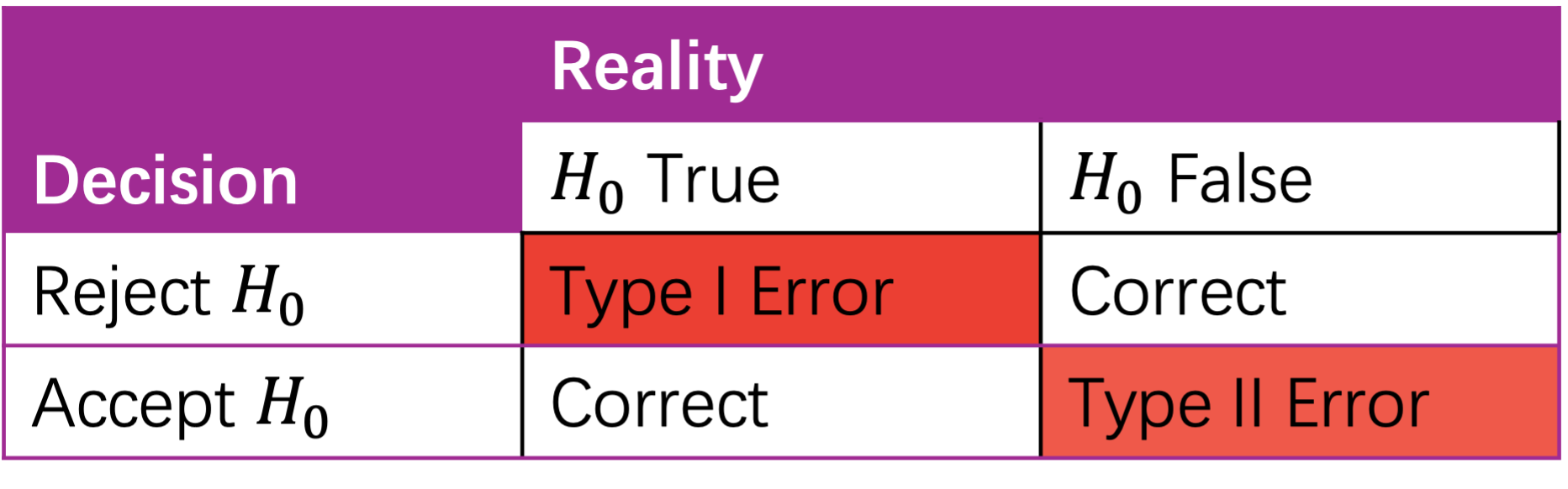
So, to formally define the two mismatch between decision and reality, we name Type I error when the null hypothesis \(H_0\) is true, but we reject it. This is also called False positive or False Alarm in other literature. Combined with the former example, that is to say when the campaign is actually not promoting sales, but due to some reason (probably insufficient sample collected / biased user group selection), we reject the null hypothesis and claim the campaign is actually effective. The Type II error is just the opposite case, where we failed to reject the null hypothesis.

With that, we can now define significance level as the greatest probability of making Type I error you are willing to tolerate. \[ \begin{align} \alpha &= \max P(\text{Type I Error})\\ &= \max P(\text{Reject } H_0 | H_0) \end{align} \] To take a more extreme example, say you are deciding whether an incoming email is spam or not. If you set the significance level \(\alpha\) to \(0\), then all emails are identified as not spam, resulting in no Type I error. If you set the significance level \(\alpha\) to \(1\), then all emails are identified as spam, every time you get a regular email you make a Type I error.

Computing p-value and make decision

Now we are at step 3 and 4, trying to make a decision based on the test statistic you calculated. But a new concept pop up, we are comparing p-value against the significance level, what is p-value?

A p-value is the probability, assuming \(H_0\) is true, that the test statistic takes on a value as extreme as or more extreme than the value observed. Denoting them in probabilistic term, we could say, p-value are as follows: 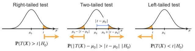Where \(T(X)\) is the Test statistic, \(t\) is the observed statistic, and \(H_0\) is our null hypothesis.

With the p-value calculated, we can then compare it with the preset significance level:

• If p-value < significance level \(\alpha\), then we reject the null hypothesis \(H_0\)
• else we don't reject the \(H_0\).

Example

Now let's dive into an concrete example to see how to perform a hypothesis testing. Let’s assume that a company claims that its employees have an average IQ of 100.

Here is the sample data we have:

• Sample Mean (\(\bar{x}\)): 103
• Population Mean (\(\mu_0\)): 100
• Standard Deviation of the Population (\(\sigma\)): 15
• Sample Size (\(n\)): 30

We suspect this average might be different, so we decide to perform a z-test with a significance level (\(\alpha\)) of 0.05 (which is a common choice in practice).

Then we calculate the z-score as test statistic: \[ z = \frac{\bar{x} - μ_0}{\frac{\sigma}{\sqrt{n}}} = \frac{103 - 100}{\frac{15}{\sqrt{30}}} = 1.095 \] Next, we'll use the z-score to find the p-value. Since our alternative hypothesis suggests the mean might be different from the population mean (i.e., a two-tailed test), we need to calculate the probability of obtaining a z-score as extreme as \(\pm 1.095\) under the null hypothesis. That is to compute the area of a standardized normal distribution using cumulative density function (CDF).

\[\text{p\_value}=2×(1−CDF(z))\] In terms of python code:

import scipy.stats import norm
p_value = 2 * (1 - norm.cdf(abs(z_score)))
>>> 0.27332167829229803

Since the p_value = 0.273 > 0.05, we failed to reject the null hypothesis. This means there is not enough evidence to conclude that the mean IQ of the company's employees is different from 100 at the 5% significance level.

Common misbeliefs

• Regarding p-value
  • The p-value represents the probability of \(H_0\) being true. WRONG!
  • A small p-value only indicates that the probability of seeing the observed data by chance is small
• Regarding conclusions
  • If we do not reject \(H_0 \rightarrow H_0\) true WRONG!
  • We can only say that there is not enough evidence.