RL00 - A glimpse of Reinforcement Learning

This post summarizes reinforcement learning from classic tabular methods to ML-based approximations and recent LLM applications like RLHF.

General definition and applications

Intuition & Definition

If you were asked, “How did you learn to ride a bike or solve a math problem?”, your answer would likely involve interaction. When learning to ride a bike, for instance, you probably didn’t follow a step-by-step guide detailing exact body movements. Instead, you engaged directly with the environment—the bike, the road, your own balance—learning through trial and error: falling, adjusting, and gradually figuring out what works. This kind of learning—driven by feedback from experience—is at the heart of reinforcement learning.

In more formal terms, reinforcement learning (RL) is learning what to do - how to map situations to actions - so as to maximize a numerical reward signal. The learner is not told which actions to take, but instead must discover which actions yield the most reward by trying them. This separates RL from supervised learning and unsupervised learning. a third paradigm

Reinforcement Learning (RL) differs from supervised learning (SL) in learning method: SL learns from a fixed dataset of labeled examples, where each input has a known correct output provided by an external supervisor. In contrast, RL learns through interaction with the environment, receiving feedback in the form of rewards rather than explicit labels, and improving behavior via trial and error. RL also differs from unsupervised learning (USL) in learning objective: USL seeks to discover hidden patterns or structures in unlabeled data (e.g., clustering or dimensionality reduction), whereas RL aims to optimize a policy that maximizes cumulative rewards.

Components

Reinforcement learning (RL) is structured around two central entities: the agent and the environment, connected through a feedback loop illustrated in the diagram 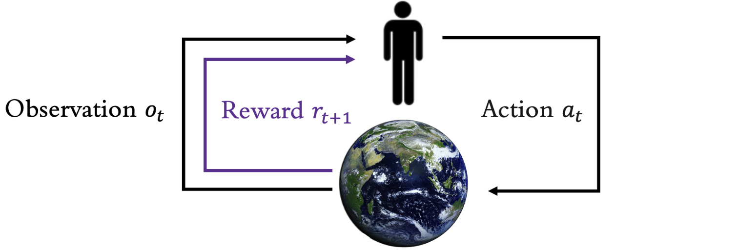At each timestep \(t\), the agent receives an observation \(o_t\) from the environment, takes an action \(a_t\), and subsequently receives a reward \(r_{t+1}\). The environment, in turn, processes the action, updates its state, and emits the next observation \(o_{t+1}\) along with the reward signal \(r_{t+1}\).

Beyond this basic interaction loop, an RL learning system comprises several core components:

• a policy \(\pi\), which maps states to actions and defines the agent's behavior;
• a reward signal, which evaluates the immediate desirability of actions taken;
• a value function, which estimates the expected cumulative reward and thus guides long-term decision-making;
• optionally, a model of the environment, which allows the agent to simulate and plan by predicting future states and rewards.

Together, these elements enable the agent to learn from experience and improve its performance over time.

Applications

Reinforcement learning shines in domains that require continuous decision-making and adaptation. In robotics, RL trains agents to control complex systems—such as robotic arms grasping objects or mobile robots navigating unpredictable terrains—through trial and error. On factory floors, it optimizes processes like automated control and supply-chain logistics, improving efficiency and resilience . In finance, RL algorithms drive algorithmic trading and portfolio management by learning strategies to buy, sell, or hold assets, maximizing risk-adjusted returns . And in gaming, RL systems such as Deep Q-Networks and AlphaZero have mastered Go, StarCraft II, and Dota 2, demonstrating extraordinary planning and strategic reasoning.

From Tabular methods to Approximated methods

Tabular solution Methods

At first glance, "tabular methods" might conjure dull images of exhaustive spreadsheets and tedious searches. So why are we still intrigued by them? Simple: they distill reinforcement learning down to its purest form, clearly revealing the fundamental mechanics behind RL algorithms.

What are the scope of tabular methods then?

We start with a basic model - Multi-armed bandits model as a representation of single state situation where value functions are introduced, along with the classical exploration vs. exploitation challenge.

Then we move on to more general problem formulation - (finite) Markov Decision Process (MDP), introducing multiple states into the problem formation. Now, our learning becomes sequential and goal-oriented, reflecting real-world decision-making as we interact repeatedly with our environment.

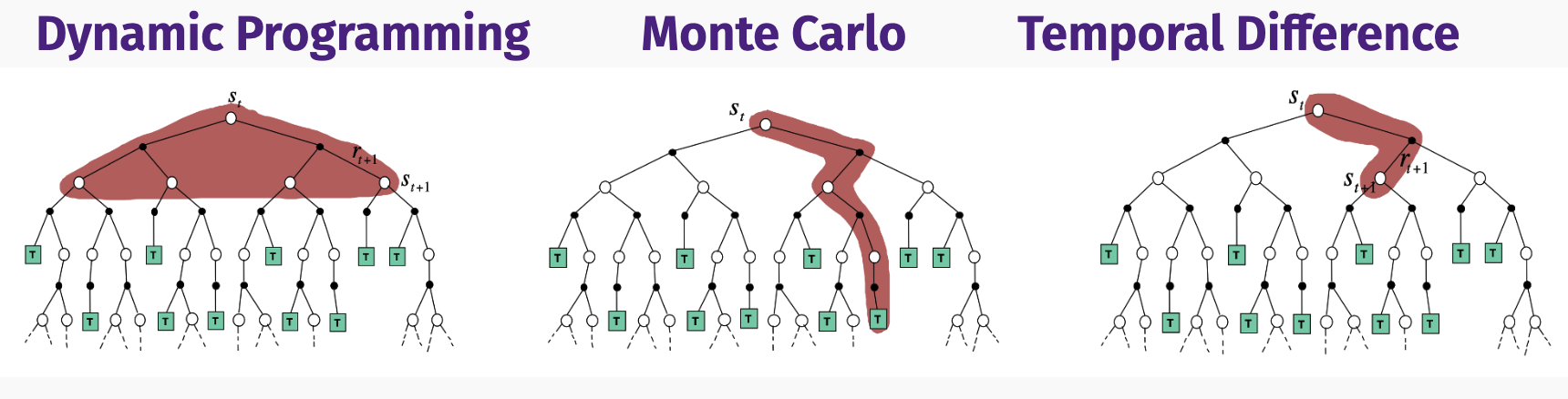
To solve MDP problem we introduced 3 new methods:

• Dynamic Programming
• Monte Carlo(MC) Method
• Temporal Difference(TD) learning

DP-vs-MC-vs-TD

As the pros and cons of each method was discovered, variation of the above 3 methods are proposed, like MC+TD via multi-step bootstrapping, TD+model learning & planning, which will be discussed in later post.

Approximate solution method

The number of distinct states grows exponentially in most realistic tasks, so storing a separate value for each state–action pair is impossible, therefore we introduced approximate solution method to search for a good approximate solution with limited computational resources.

The problem with large state spaces is not just the memory needed for large tables, but the time and data needed to fill them accurately. In many of our target tasks, almost every state encountered will never have been seen before. This propose challenges to the policy's generalization capability. As key RL components are all functions:

• State update functions map observations to states
• Value functions map states to values
• Policies map states to actions
• Models map states and actions to next states and rewards. to achieve generalization, we can reuse the tool - function approximation - studied in supervised learning.

There are a bunch of function approximator can be used:

• state aggregation (feature engineering) - represent state by a feature vector
• linear function (regression, nearest-neighbors, etc)
  • tabular function (look-up tables) are special case where \(n\) = number of states and where \(w_i\) is the value of each state \(s_i\). \[ v_{\mathbf w}(s)= \begin{bmatrix} w_1\\ \vdots\\ w_n \end{bmatrix}^{\top} \begin{bmatrix} \mathbf 1\!\left(s=s_1\right)\\ \vdots\\ \mathbf 1\!\left(s=s_n\right) \end{bmatrix} \]
• non-linear function (neural network, decision tree, etc)

As for the general methodology, we can approximate value function:

• On-policy semi-gradient TD & SARSA
• Deep Q-Network (DQN)
• Experience-replay variants

or perform direct policy approximate:

• REINFORCE (Monte-Carlo Policy Gradient) & other policy-gradient methods
• Trust-Region Policy Optimisation (TRPO) series
  • TRPO enforces a KL-divergence trust region via conjugate-gradient solving.
  • Proximal Policy Optimisation (PPO) – replaces TRPO’s constraint with a simple clip or penalty surrogate; the current default in many toolkits.
• Deterministic Policy Gradient (DPG) & Deep DPG (DDPG) – actor outputs a deterministic action; critic supplies its gradient, enabling continuous-action control.
• Advantage Actor–Critic (A2C/A3C) – many lightweight actors share a global critic (or run asynchronously) to parallelise on-policy learning.

RL nowadays

RL with Deep Learning

Deep learning has super-charged reinforcement learning by providing expressive neural representations for policies, value functions, and environment models. Trajectory Transformer (Janner et al., NeurIPS 2021) shows how discretising continuous trajectories into tokens effectively quantises the state-action space, letting a plain Transformer do offline planning via sequence modelling, also brought the influential Transformer work into RL context.

Meanwhile, Dyna-style architectures integrate model-free Q-learning with a learned neural world-model whose simulated roll-outs supply extra training data, blending model-based and model-free updates in one deep RL loop.

At the high end, AlphaGo and its successor AlphaZero couple deep convolutional policy/value nets with Monte-Carlo tree search and self-play, achieving super-human performance in Go, chess, and shogi—powerfully illustrating how CNN features and scalable RL jointly push decision-making beyond human expertise.

RL with Large Language Models

Reinforcement Learning (RL), once a niche playground for gamers and simulation enthusiasts aiming for super-human performance in video games, has burst into the mainstream by joining forces with Large Language Models (LLMs). Techniques such as RLHF, RLAIF, and RLVR have transformed RL from a specialized skillset into a crucial step toward training the next generation of AI—accelerating progress in the pursuit of AGI. As RL insights merge seamlessly with LLMs, a dynamic new era in artificial intelligence is unfolding, where machines not only learn but actively align with human values, preferences, and intentions.