An introduction to KMP algorithm

In this post, I will introduce the string matching problem, and a clever solution - KMP algorithm. I start from the brute force method and showed how to deduce KMP.

Introduction

String Matching Problem

• Given strings S(length m) and T (length n), find T in S. The string T called pattern.
• Wide Applications, essential role in various real-world problems.
  • Text processing: spell checking, text classification, information retrieval (especially in NLP field).
  • Pattern recognition: bioinformatics, speech recognition
  • Database management: used to searching and retrieving efficiently.

KMP algorithm

• This is an algorithm designed for the above problem, which is time efficient.
• Summary of key ideas in KMP (for those are familiar with string matching problem):
  • reduce the total comparison round --> utilize the information gained after each failed comparison
  • exploit the information of the pattern string --> maintain an array for storing useful information.

Brute Force method

• Before dig into KMP algorithm, let's look at the method which defines the lower limit of the performance.

  # Brute force algorithm for string matching
  def bruteForce(S, P):
    for i in range(len(S) - len(P) + 1):
      if S[i : i + len(P)] == P:
        print(f'Find a matching point at position {i}') # f-string

  void bruteForce(char *s, char *p) {
    int lenS = strlen(s), lenP = strlen(p);
    
    for(int i = 0; i <= lenS - lenP; i++) {
    	boolean flag = true;
      
      for int(j = 0; p[j] != '\0'; j++) {
        if(s[i+j] != p[j]) {
          flag = false;
          break;
        }
      }
      
      if(flag) printf("Find a matching point at position %d\n", i);
    }
  }

• The intuition is pretty straight forward,
  • 1. we match the string character by character, if no failed matching till the end of the pattern string, then a successful matching was found.
    2. Then for the entire string, we place the pattern string at the start of each character in S string, then perform the above the step.

Analysis

• The step 1 takes |P| (length of pattern string, usually marked as n) time, and the step 2 takes |S| (length of original string) time, we could easily conclude the time complexity is \(O(|P| \cdot |S| )\).
• Why is it so slow? Or where could we improve?
  • Apparently we could not optimize the comparison process at step 1 , to check a match we need to perform a full comparison.
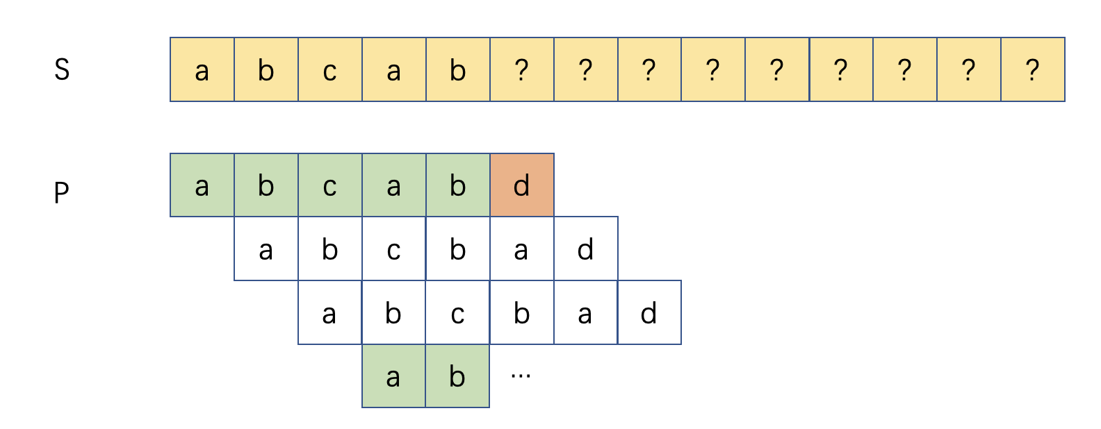
  • Naturally we turned to think if we could reduce the round for matching in step 2. Look at the example below:

    • 

      image.png

    • After the above failed comparison, the brute force would start a new round of comparison at S[1],S[2]. These attempts is obvious to fail. The KMP algorithm therefore proposes a mechanism to skip these impossible matching.
    • The resulting process should be like this: (white colored means comparison skipped):

    • 

      image.png

Deducing the KMP algorithm

Partial Matching Table

• Following the intuition of skipping impossible matching, we need to find a mechanism to decide which ones should be skipped. The KMP algorithm proposed a structure called partial matching table, which stores the information we need.
  • The partial matching table has the same length as the pattern string, denoted as next[]. Given the length of P is n, next[i] represents
    • If substring p[0..i] has a pair of identical prefix and suffix (p[0..k-1] == p[i-(k-1),..i]), then next[i] = k
    • For example
      • for the pattern string abcabcd,we have next[i] = [0,0,0,1,2,3,0]. When i = 5, the string is abcabc, therefore we could get identical pair abc, where the length is 3
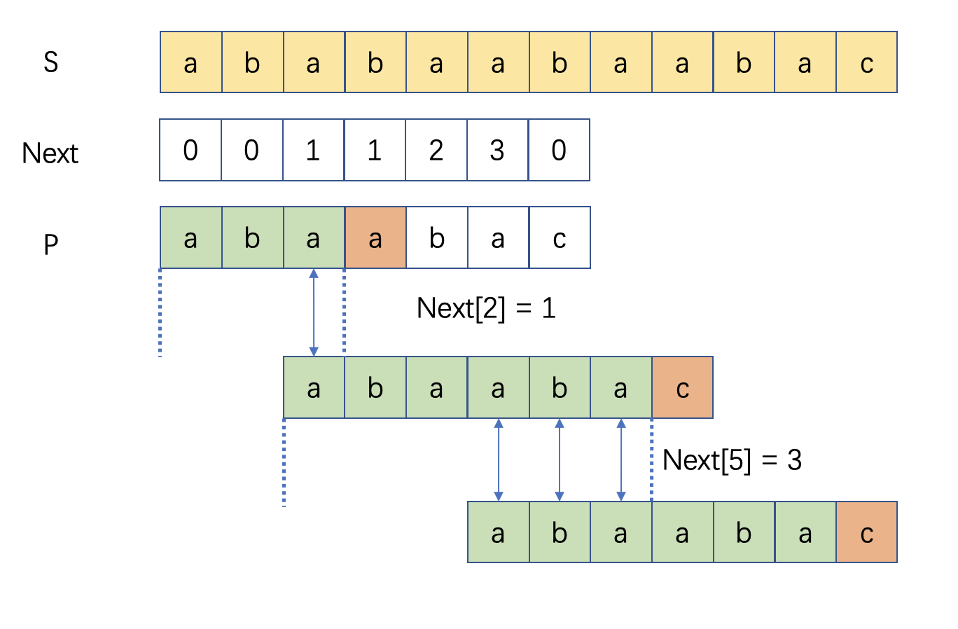
• You may have noticed, with next[] array calculated, we could skip impossible matchings by referencing the next[] array. As shown in below example

  • 

    image.png

  • When we failed the first match at P[3], we replace the P[1] on the mismatched index and restart the matching. When failed the second match at P[6], we replace P[3] on the mismatched index.
  • From above we could conclude, we utilize the identical prefix and suffix for skipping some comparisons. Say the mismatch occurs at P[i], then between P[0]~P[i-1], the former next[i-1] character(s) should be the same as the latter next[i-1] character(s), so we could replace the suffix with the prefix. In conclusion, we could realign P[next[i-1]] with P[i].
  • In other word, the next[] array provides reference for how to skip comparison and how many comparison to skip.

    # Suppose we have calculated the next[] array
    def search():
      s_pointer = 0
      p_pointer = 0
      
      while s_pointer < len(s):
        if s[s_pointer] == p[p_pointer]: # If matched, increment both pointers
          s_pointer += 1
          p_pointer += 1
        elif p_pointer: 				# mismatched at p[p_pointer], move p_pointer
          p_pointer = next[p_pointer-1]
        else:							# mismatcher at p[0]
          s_pointer += 1
          
        if p_pointer == len(p):
          print(f'The matching start point is {s_pointer - p_pointer}')
          p_pointer = next[p_pointer - 1]
          

  • How to analysis the complexity of this step?
    • We could use amortized analysis, the s_pointer could increment at most len(s) times, therefore the time complexity is \(O(n)\).

Calculating Partial Matching Table

• Now we have drawn the overall picture of KMP algorithm. The only problem remained is how to calculate the next[] array.

• An easy way to come up with:

  def calNext(x):
    for i in range(x, 0, -1):
      if p[0:i] == p[x+1-i : x+1]: # Note that p[0..x] has length x+1
        return i
    return 0
  
  next = [calNext(x) for x in range(len(p))]

  • However, the complexity of algorithm is \(O(m^2)\), as for each entry x , we perform x times check.

• An optimized way, consider using recursion.

  • Suppose we already know next[x-1], we want to calculate next[x]
    • if P[x] == P[next[x-1]] --> next[x] = next[x-1] + 1
    • if P[x] != P[next[x-1]]
      • To simply, we denote next[x-1] as pre

      • 

        image.png

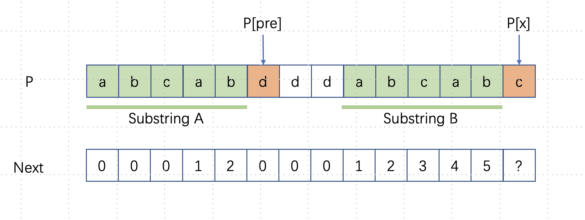
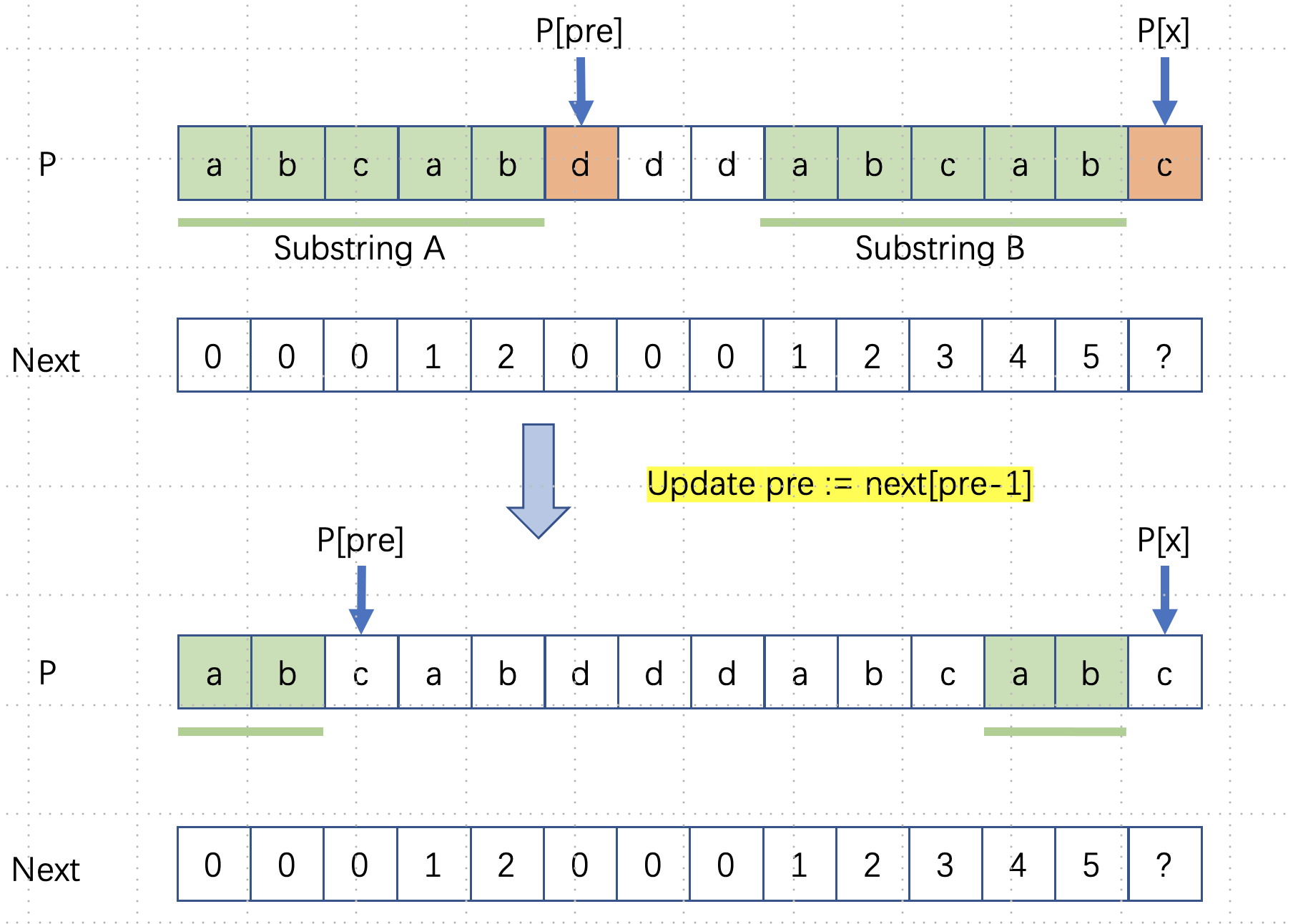
      • When this two character does not match, we should shorten the pre and try the match again. We could utilize the property of next[] array - P[0]~P[pre - 1] (A) is identical to P[x - pre] ~ P[x-1] (B).
      • To shorten pre, we need to find the a k, which maximizes the length, where prefix(A,k) == suffix(B,k).
      • Remember A and B is identical, then we transform the problem to find the longest common prefix and suffix of A! which is exactly next[pre-1].

      • 

        image.png

      • Therefore we conclude: Iterate pre = next[pre-1], until P[next[x-1]] == P[x]

        next = []
        
        def calNext():
          next.append(0)	# Base case
          x = 1
          pre = 0
          
          while x < len(p):
            if p[pre] == p[x]: 
              pre += 1
              x += 1
            elif pre:
              pre = next[pre-1]
            else:
              next.append(0)
              x += 1

      • We could find the code looks similar to the one developed earlier. It is because they actually share the same essence. search() method perform string matching between S and P, where calNext() perform string matching between P and P!
      • Similar to previous algorithm, the time complexity is \(O(m)\).

• In conclusion, we conquer the string matching problem with time complexity \(O(m+n)\)!

• Salute to the designers of this algorithm: Donald Knuth(K), James H. Morris(M), Vaughan Pratt(P).

References

• Chinese Explanation of this Algorithm
• KMP algorithm - WikiPedia